The unpredictability behind the simplest functions
The beauty of math lies in its universality, the way that so many seemingly unrelated concepts relate to each other. For instance, what if I asked you, “what do rabbit populations and a leaky faucet have in common?” This may sound like a setup for one of the worst jokes in history, but I assure you, it is not. What unifies these two vastly different concepts is chaos.
Chaos is a phenomenon found in mathematics and science, where rule-based systems, also known as deterministic systems, behave unpredictably (1). Deterministic systems are systems where every output can be precisely determined from their input. While some of these systems, such as the equation y = 2x, may be governed by simple and precise rules, their outcomes are largely unpredictable in the long run.
But, before we examine an example of a chaotic system, we need to understand the basics of iteration. In Algebra 1, we learned about functions. We take an input, x, and plug it into a function, f; the output of f(x) is y. Iteration is the process of continually repeating this process, feeding the output, y, back into the function f, to create a new output: f(y).
The population of a rabbit colony from year to year is an example of an iterable deterministic system because the rabbit population of each year depends on that of the last. We can use the logistic equation to model this rabbit growth: f(x) = rx(1-x), where f(x) represents the rate at which the rabbit population is changing; for example, if f(x) = 2, the rabbit population is doubling yearly.
To solve this equation, we need to understand what each variable means. X represents the proportion of the current number of rabbits to the maximum possible population of rabbits. This maximum, also known as the carrying capacity, is determined by factors such as the availability of food or other environmental factors. The variable r represents the estimated number of offspring each rabbit will have.
You may wonder, why is (1-x) included in the equation? If the rabbit population reaches the carrying capacity, x will equal one, making the right-hand side of the equation equal to zero; thus, the population is not growing (1). Essentially, the (1-x) guarantees that the population cannot surpass the carrying capacity. Now that we understand the basics of logistics equations, let us examine the behavior of rabbit populations with different rates of reproduction.
A big part of mathematics is experimenting with different values, so we will plot some iterations of the logistic equation for some values r in a time series plot. The x-axis in this diagram will show the time, which will be how many times the equation has been iterated. The y-axis in this diagram will show the value of x, which is the proportion of the current number of rabbits to the carrying capacity. The time series plot of the logistic equation for r = 1.5 is seen in Graph 1. Examining the graph, the values of x appear to stay constant at around 0.33 after nine iterations. Were this to play out in the real world, the rabbits—who are producing 1.5 offspring each—would have their population settle at one-third of the maximum after nine years. This is what is known as the end-state of the function: where the value of x goes as the number of iterations approach infinity.

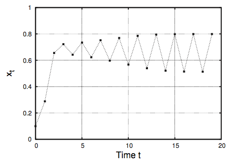
Next, we will repeat this process with r = 3.2; this time series plot is seen in Graph 2. The values of x seem to bounce between 0.5 and 0.8. Because it will do this indefinitely, the end-states are 0.5 and 0.8.

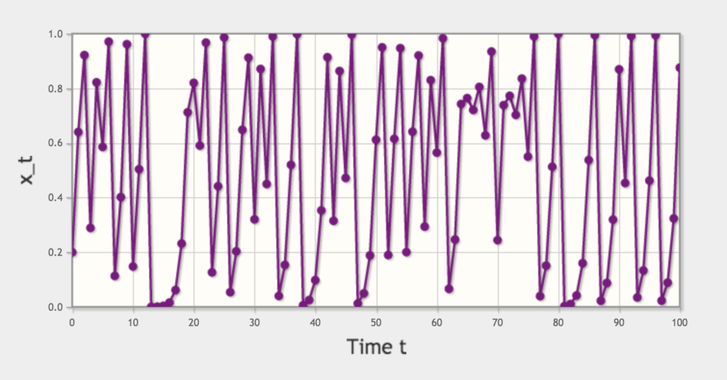
But when we set r = 4, something interesting happens. After iterating this function, f(x) = 4x(1-x), we graph the results in the time-series plot in Graph 3. Unlike in the time-series plots at other values of r, in this graph, the values of x never seem to settle down. Because there is no pattern to the values of x, there is no end-state (2). This graph exhibits chaos: a completely deterministic function that has an unpredictable outcome.

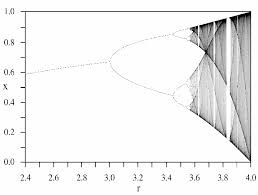
The end-states for all logistic equations of 1 < r < 4 can be expressed in what is known as a bifurcation diagram, as seen in Graph 4. Here, the end states are displayed on the y-axis, and r is shown on the x-axis. Observing the trends of Graph 4, one branch of end-state values appears to split into two at around r = 3. These two branches then both split again at around r = 3.4. This process of splitting is known as period-doubling, which continues until r = 4, when the graph becomes aperiodic and chaotic. The bifurcation diagram stops at r = 4 because when r > 4, the values of x exceed one or drop below zero, which does not make sense in the context of the problem—the population cannot exceed the carrying capacity or be negative.

The properties of aperiodicity can be found in other places than on paper or on a computer simulation. Aperiodic behavior exists everywhere, even in a kitchen sink. The rate at which a faucet drips obviously increases with the rate of water flow. As the knob turns and the flow rate of the faucet increases, the drip rate will undergo period-doubling before reaching a chaotic state, when there is no way to predict when the next drop will come.
Examining chaos with simple deterministic functions shows that advanced knowledge of calculus is not required to understand interesting mathematical concepts. This only highlights the beauty of mathematics: it exists at the intersection of seemingly unrelated phenomena.
– Timothy Guan
References
- Feldman, D. P. (2014). Chaos and fractals an elementary introduction. Oxford: Oxford Univ. Press.
- Guo, Justin. 2014, Sept., 10. ANALYSIS OF CHAOTIC SYSTEMS. UChicago. http://math.uchicago.edu/~may/REU2014/REUPapers/Guo.pdf
Images
- Feldman, David. P. 2012. Chaos and fractals an elementary introduction. Oxford
- Source: Feldman, David. P. 2012. Chaos and fractals an elementary introduction. Oxford
- http://chaos.coa.edu/time_series.html
- https://geoffboeing.com/2015/03/chaos-theory-logistic-map/


Be First to Comment